
Multigrid#
These examples are based on code originally written by Krzysztof Fidkowski and adapted by Venkat Viswanathan. This page also contains figures from Krzysztof Fidkowski’s CFD course notes.
import time
import numpy as np

import matplotlib.pyplot as plt
import niceplots

plt.style.use(niceplots.get_style())
niceColors = niceplots.get_colors_list()

# Force the jupyter notebook to use vector graphics
import matplotlib_inline

matplotlib_inline.backend_inline.set_matplotlib_formats("pdf", "svg")
In this problem we’re going to solve the same 1D heat transfer problem as the past 2 weeks’ example, this time using multigrid.
First let’s redefine the problem and some of the functions we used to iteratively solve it
# Define the parameters
L = 2.0  # Length of domain
kappa = 0.5  # Thermal conductivity
Nx = 64  # Number of intervals
T0 = 1.0  # Left boundary condition
TN = 4.0  # Right boundary condition
tol = 1e-6  # Tolerance for iterative solver


# Define the symbolic function q(x)
def q(x, L):
    return np.sin(np.pi * x / L)


def computeResidual(u, q, kappa, dx):
    """Compute the residual of the 1D heat equation

    Parameters
    ----------
    u : numpy.ndarray
        Current state vector
    q : numpy.ndarray
        Source term vector
    kappa : float
        Thermal conductivity
    dx : float
        Grid spacing

    Returns
    -------
    numpy.ndarray
        Residual vector
    """
    dx2 = dx**2
    r = np.zeros_like(u)
    r[1:-1] = kappa * (u[:-2] - 2 * u[1:-1] + u[2:]) / dx2 + q[1:-1]

    return r


def computeNorm(r):
    """Compute the "normalized" norm of a vector

    Parameters
    ----------
    r : numpy.ndarray
        Vector to compute the norm of
    """
    return np.linalg.norm(r) / np.sqrt(len(r))


def iterativeSolve(u, q, kappa, dx, smootherFunc, omega=1.0, tol=1e-4, maxIter=5000):
    """Iteratively solve the steady-state 1D heat equation

    Parameters
    ----------
    u : numpy ndarray
        Initial state
    q : numpy ndarray
        Right-hand side
    kappa : float
        Thermal conductivity
    dx : float
        Grid spacing
    smootherFunc : function with signature f(u, q, kappa, dx, omega=1.0))
        Function that performs a single smoothing iteration
    omega : float, optional
        Relaxation factor, by default 1.0
    tol : float, optional
        Residual norm to stop at, by default 1e-4
    maxIter : int, optional
        Maximum number of iterations, by default 5000

    Returns
    -------
    numpy ndarray
        New state
    """
    resNormHistory = []
    iterationTimes = []
    printFrequency = max(1, maxIter // 10)
    startTime = time.time()
    for ii in range(maxIter):
        r = computeResidual(u, q, kappa, dx)
        resNorm = computeNorm(r)
        if ii % printFrequency == 0:
            print(f"Iteration {ii}: Res norm = {resNorm:.2e}")
        resNormHistory.append(resNorm)
        iterationTimes.append(time.time() - startTime)
        if resNorm < tol or resNorm > 1e10 or np.isnan(resNorm):
            break
        u = smootherFunc(u, q, kappa, dx, omega=omega)

    if ii % printFrequency != 0:
        print(f"Iteration {ii}: Res norm = {resNorm:.2e}")
    return u, resNormHistory, iterationTimes


def gaussSeidelIteration(u, q, kappa, dx, omega=1.0):
    """Perform one Gauss-Seidel smoothing step

    Parameters
    ----------
    u : numpy.ndarray
        Current state vector
    q : numpy.ndarray
        Source term vector
    kappa : float
        Thermal conductivity
    dx : float
        Grid spacing
    omega : float, optional
        Relaxation factor, by default 1.0

    Returns
    -------
    numpy.ndarray
        Updated state vector
    """
    dx2k = dx**2 / kappa
    uNew = u.copy()
    for ii in range(1, len(u) - 1):
        uNew[ii] = omega * (0.5 * (uNew[ii - 1] + uNew[ii + 1] + q[ii] * dx2k)) + (1.0 - omega) * uNew[ii]
    return uNew
The effectiveness of multigrid depends on two things:
Iterative smoothers require fewer iterations when started from a good initial guess
Iterative smoothers reduce high frequency errors faster than low frequency errors
Let’s demonstrate these 2 points, first by solving the problem starting from a bad initial guess (\(T=0\) everywhere) and then by solving the problem starting from a good initial guess (\(T\) varying linearly between the boundaries).
T_init_good = np.linspace(T0, TN, Nx + 1)
T_init_bad = np.copy(T_init_good)
T_init_bad[1:-1] = 0.0

x = np.linspace(0, L, Nx + 1)
q_array = q(x, L)

T_sol_bad, res_history_bad, iter_times_bad = iterativeSolve(
    T_init_bad, q_array, kappa, L / Nx, gaussSeidelIteration, omega=1.4, tol=tol
)
T_sol_good, res_history_good, iter_times_good = iterativeSolve(
    T_init_good, q_array, kappa, L / Nx, gaussSeidelIteration, omega=1.4, tol=tol
)
Iteration 0: Res norm = 2.62e+02
Iteration 500: Res norm = 2.18e-01
Iteration 1000: Res norm = 1.30e-02
Iteration 1500: Res norm = 7.76e-04
Iteration 2000: Res norm = 4.63e-05
Iteration 2500: Res norm = 2.76e-06
Iteration 2680: Res norm = 9.99e-07
Iteration 0: Res norm = 7.02e-01
Iteration 500: Res norm = 4.24e-02
Iteration 1000: Res norm = 2.53e-03
Iteration 1500: Res norm = 1.51e-04
Iteration 2000: Res norm = 8.99e-06
Iteration 2390: Res norm = 9.97e-07
fig, ax = plt.subplots()
ax.set_yscale("log")
ax.set_xlabel("Iteration")
ax.set_ylabel("$||r||_2$")
ax.plot(res_history_bad, clip_on=False, label="Bad initial guess")
ax.plot(res_history_good, clip_on=False, label="Good initial guess")
ax.axhline(tol, color="Gray", linestyle="--", label="Tolerance")
ax.legend(labelcolor="linecolor")
niceplots.adjust_spines(ax)

To demonstrate how different frequencies of error are reduced at different rates, we’ll run 10 iterations starting from the true solution plus a high frequency error and then starting from the true solution plus a low frequency error.
T_init_highfreq = T_sol_good + 0.01 * np.sin(8 * np.pi * x / L)
T_init_lowfreq = T_sol_good + 0.01 * np.sin(1 * np.pi * x / L)

T_sol_lowfreq, res_history_lowfreq, iter_times_lowfreq = iterativeSolve(
    T_init_lowfreq, q_array, kappa, L / Nx, gaussSeidelIteration, omega=1.2, tol=1e-14, maxIter=10
)
T_sol_highfreq, res_history_highfreq, iter_times_highfreq = iterativeSolve(
    T_init_highfreq, q_array, kappa, L / Nx, gaussSeidelIteration, omega=1.2, tol=1e-14, maxIter=10
)

fig, ax = plt.subplots()
ax.set_xlabel("x")
ax.set_ylabel(r"$T - T_{sol}$")
ax.plot(x, T_init_highfreq - T_sol_good, "--", c=niceColors[0], label="Initial guess", clip_on=False)
ax.plot(x, T_init_lowfreq - T_sol_good, "--", c=niceColors[1], clip_on=False)
ax.plot(x, T_sol_highfreq - T_sol_good, c=niceColors[0], label="After 10 iterations", clip_on=False)
ax.plot(x, T_sol_lowfreq - T_sol_good, c=niceColors[1], clip_on=False)
ax.legend(ncol=2, loc="lower right", bbox_to_anchor=(1.0, 1.0))
niceplots.adjust_spines(ax)
Iteration 0: Res norm = 8.65e-03
Iteration 1: Res norm = 8.62e-03
Iteration 2: Res norm = 8.59e-03
Iteration 3: Res norm = 8.56e-03
Iteration 4: Res norm = 8.53e-03
Iteration 5: Res norm = 8.50e-03
Iteration 6: Res norm = 8.47e-03
Iteration 7: Res norm = 8.44e-03
Iteration 8: Res norm = 8.41e-03
Iteration 9: Res norm = 8.38e-03
Iteration 0: Res norm = 5.47e-01
Iteration 1: Res norm = 4.63e-01
Iteration 2: Res norm = 3.90e-01
Iteration 3: Res norm = 3.27e-01
Iteration 4: Res norm = 2.75e-01
Iteration 5: Res norm = 2.30e-01
Iteration 6: Res norm = 1.93e-01
Iteration 7: Res norm = 1.61e-01
Iteration 8: Res norm = 1.34e-01
Iteration 9: Res norm = 1.12e-01

Implementing a basic 2-level multigrid solver#
In this example we are going to implement a very simple 2-level multigrid smoother to use in out iterative solver algorithm. Note that this is not a great implementation, it is hardcoded to use only 2 levels. In your next homework you will be given the task of implementing a more general multigrid solver that can use any number of levels.
A 2-level multigrid iteration consists of the following steps:
Running \(n_\text{pre}\) iterations of a smoother on the fine grid
Restricting/averaging the residual to the coarse grid
Running \(n_\text{coarse}\) iterations of a smoother on the coarse grid
Prolonging/interpolating the coarse grid correction to the fine grid
Adding the fine grid correction to the solution
Running \(n_\text{post}\) iterations of a smoother on the fine grid
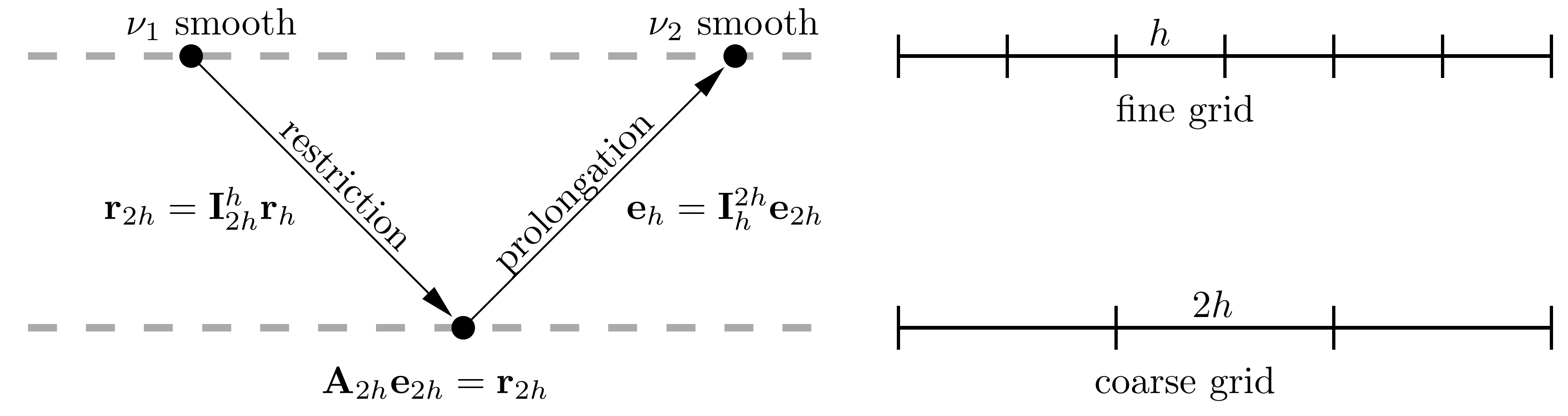
It’s important to recognise that the system of equations we are solving on the coarse grid is slightly different from the system we are solving on the fine grid. On the fine grid we are solving:
Once we solve the system on the coarse grid, one thing we could do is just to interpolate the coarse grid solution back to the fine grid, overwriting whatever we had on the fine grid. However, this would not be a good idea as we would be throwing away information we had on the fine grid. Instead, we want to use the coarse grid to compute a correction to our fine grid solution.
To help think about how to compute this correction, let’s define the solution error:
where \(T^*\) is the true solution and \(T\) is our current approximation to the solution. Notice that if we knew what \(e\) was, we could just add it to \(T\) to get the true solution.
If we multiply the error by our finite difference matrix \(A\), we get:
So on the coarse grid, we solve \(Ae = r\) approximately. to find a correction \(e\) that should take us closer to the true solution, \(T^*\) on the coarse grid. Once we have this correction, we can interpolate it back to the fine grid and add it to our current approximation to the solution there.
In this implementation, our coarse grid is exactly a factor of 2 coarser that the fine grid, the stencils for the restriction and prolongation operators are therefore pretty simple, as shown below. In more complex codes, it may not be possible generate such an ideal coarse grid and the restriction and prolongation may be more complex averaging/interpolation operations.
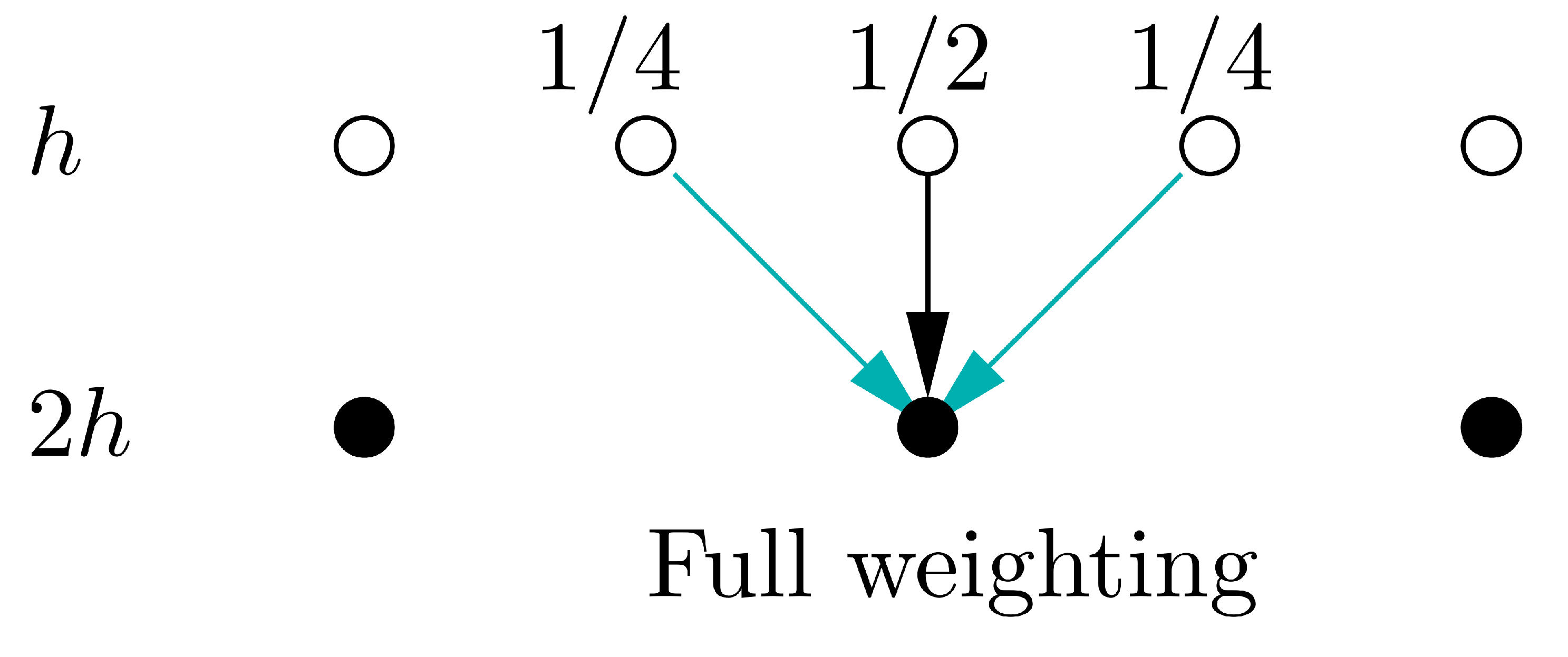
# Define residual restriction operator from fine grid to coarse grid using full-weighting
def restrict_to_coarse(r_fine):
    r_coarse = np.zeros((len(r_fine) - 1) // 2 + 1)  # Create an empty coarse grid
    for ii in range(1, len(r_coarse) - 1):
        r_coarse[ii] = 0.25 * r_fine[2 * ii - 1] + 0.5 * r_fine[2 * ii] + 0.25 * r_fine[2 * ii + 1]
    return r_coarse
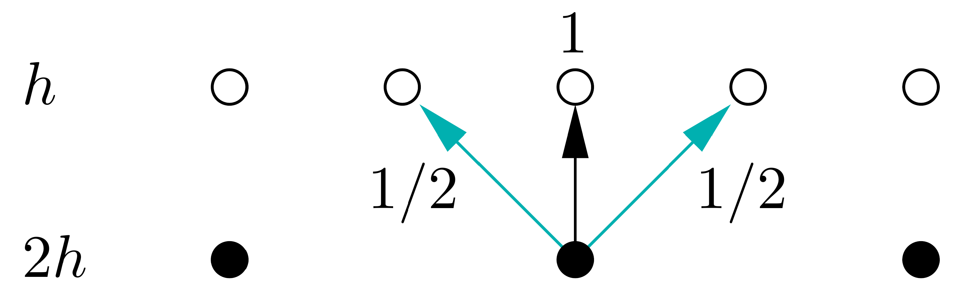
# Define prolongation operator from coarse grid to fine grid
def prolongate_to_fine(u_coarse):
    u_fine = np.zeros(2 * (len(u_coarse) - 1) + 1)  # Create an empty fine grid
    # Assign values from coarse grid directly for even elements
    u_fine[2:-2:2] = u_coarse[1:-1]
    # Use weights 1/2 and 1/2 for odd elements
    u_fine[1:-1:2] = 0.5 * (u_coarse[:-1] + u_coarse[1:])
    return u_fine
def multigridIteration(u, q, kappa, dx, omega=1.0, num_pre=1, num_post=1, num_coarse=2):
    u_new = u.copy()
    # Pre-smoothing iterations
    for _ in range(num_pre):
        u_new = gaussSeidelIteration(u_new, q, kappa, dx, omega=omega)

    # Compute the residual
    r = computeResidual(u_new, q, kappa, dx)

    # Restrict the residual to the coarse grid
    r_coarse = restrict_to_coarse(r)

    # Smooth the error on the coarse grid
    du_coarse = np.zeros_like(r_coarse)
    for _ in range(num_coarse):
        du_coarse = gaussSeidelIteration(du_coarse, r_coarse, kappa, 2 * dx, omega=omega)

    # Prolongate the state update to the fine grid and add to the current solution
    du_fine = prolongate_to_fine(du_coarse)
    u_new += du_fine

    # Post-smoothing iterations
    for _ in range(num_post):
        u_new = gaussSeidelIteration(u_new, q, kappa, dx, omega=omega)

    return u_new
num_pre = 1
num_post = 1
num_coarse = 2

# Compute how much work each multigrid iteration takes compared to a single GS iteration on the fine grid
multigrid_work = 0.5 * num_coarse + num_pre + num_post

num_iters = int(10 / multigrid_work)

T_sol_lowfreq, res_history_lowfreq, iter_times_lowfreq = iterativeSolve(
    T_init_lowfreq, q_array, kappa, L / Nx, multigridIteration, omega=1.2, tol=1e-14, maxIter=num_iters
)
T_sol_highfreq, res_history_highfreq, iter_times_highfreq = iterativeSolve(
    T_init_highfreq, q_array, kappa, L / Nx, multigridIteration, omega=1.2, tol=1e-14, maxIter=num_iters
)
Iteration 0: Res norm = 8.65e-03
Iteration 1: Res norm = 8.37e-03
Iteration 2: Res norm = 8.08e-03
Iteration 0: Res norm = 5.47e-01
Iteration 1: Res norm = 2.47e-01
Iteration 2: Res norm = 1.10e-01
fig, ax = plt.subplots()
ax.set_xlabel("x")
ax.set_ylabel(r"$T - T_{sol}$")
ax.plot(x, T_init_highfreq - T_sol_good, "--", c=niceColors[0], label="Initial guess", clip_on=False)
ax.plot(x, T_init_lowfreq - T_sol_good, "--", c=niceColors[1], clip_on=False)
ax.plot(x, T_sol_highfreq - T_sol_good, c=niceColors[0], label=f"After {num_iters} iterations", clip_on=False)
ax.plot(x, T_sol_lowfreq - T_sol_good, c=niceColors[1], clip_on=False)
ax.legend(ncol=2, loc="lower right", bbox_to_anchor=(1.0, 1.0))
niceplots.adjust_spines(ax)

Now let’s see how fast multigrid converges from the bad initial guess compared to plain Gauss-Seidel.
When comparing the number of iterations required for convergence, we need to account for the fact that each multigrid iteration is more expensive than a Gauss-Seidel iteration.
T_sol_bad_gs, res_history_bad_gs, iter_times_bad_gs = iterativeSolve(
    T_init_bad, q_array, kappa, L / Nx, gaussSeidelIteration, omega=1.4, tol=tol
)
T_sol_bad_mg, res_history_bad_mg, iter_times_bad_mg = iterativeSolve(
    T_init_bad, q_array, kappa, L / Nx, multigridIteration, omega=1.4, tol=tol
)
Iteration 0: Res norm = 2.62e+02
Iteration 500: Res norm = 2.18e-01
Iteration 1000: Res norm = 1.30e-02
Iteration 1500: Res norm = 7.76e-04
Iteration 2000: Res norm = 4.63e-05
Iteration 2500: Res norm = 2.76e-06
Iteration 2680: Res norm = 9.99e-07
Iteration 0: Res norm = 2.62e+02
Iteration 269: Res norm = 9.45e-07
# Scale the multigrid iteration count by the amount of work each iteration takes
mg_iterations = np.arange(len(res_history_bad_mg)) * multigrid_work

fig, ax = plt.subplots()
ax.set_yscale("log")
ax.set_xlabel("Equivalent fine-grid iterations")
ax.set_ylabel("$||r||_2$")
ax.plot(res_history_bad_gs, clip_on=False, label="Gauss-Seidel")
ax.plot(mg_iterations, res_history_bad_mg, clip_on=False, label="Multigrid")
ax.axhline(tol, color="Gray", linestyle="--", label="Tolerance")
ax.legend(labelcolor="linecolor")
niceplots.adjust_spines(ax)
